In the previous section we have seen how to apply the variational method to a simple simgle-particle problem. As we treat more complicated problems, such as heavier atoms, molecules, and ultimately, solids, the complexitiy increases as the number of particles, and degrees of freedom increases. In these so-called, many-body problems, we have to consider the motion of the nuclei, the interaction between the protons and electrons, and between electrons themselves.
We will consider a general system of ![]() nuclei described by coordinates,
nuclei described by coordinates,
![]() , momenta,
, momenta,
![]() , and masses
, and masses ![]() , and
, and ![]() electrons described by coordinates,
electrons described by coordinates,
![]() , momenta,
, momenta,
![]() , and spin variables,
, and spin variables,
![]() . The Hamiltonian of the system is given by
. The Hamiltonian of the system is given by
 |
(49) | ||
 |
(50) | ||
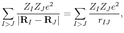 |
(51) | ||
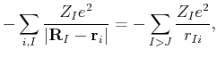 |
(52) | ||
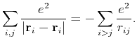 |
(53) |
A second approximation is to assume that the wave-function of the many-electron system takes the form of an antisymmetized product of one-electron wave-functions (remember that electrons are fermions). This simplification transforms the complicated many-body problem into the problem of a single-particle in an effective "mean-field" potential determined by the positions of the other electrons. This is the basic idea behind the Hartree-Fock method.
We can immediatley make two obervations: The first is that we are assuming that the physics can be described by single-particle wave-functions, and therefore, thsi corresponds to approximating the actual ground state by a variational ansatz. As a consequence, all the concepts learned in the previous section will apply here as well. A second observation is that the effective potential feld by the electrons will have to be calculated self-consistently: every time we update or modify the single particle wave-function, the potential will have to be updated as well.
We shall see that in this variational approach, correlations between electrons are neglected to some extent. In particular, Coulomb repulsion between electrons is taken into account in an averaged way.