The Born-Oppenheimer approximation

The Born-Oppenheimer Approximation is the assumption that the electronic motion and the nuclear motion in molecules can be separated. It leads to a molecular wave function in terms of electron positions and nuclear positions.

This involves the following assumptions:

$\bullet$ The electronic wavefunction depends upon the nuclear positions but not upon their velocities, i.e., the nuclear motion is so much slower than electron motion that they can be considered to be fixed.

$\bullet$ The nuclear motion (e.g., rotation, vibration) sees a smeared out potential from the speedy electrons.

We know that if a Hamiltonian is separable into two or more terms, then the total eigenfunctions are products of the individual eigenfunctions of the separated Hamiltonian terms, and the total eigenvalues are sums of individual eigenvalues of the separated Hamiltonian terms.

Consider, for example, a Hamiltonian which is separable into two terms, one involving coordinate $q_1$ and the other involving coordinate $q_2$.

$${H} = {H}_1(q_1) + {H}_2(q_2)$$

with the overall Schrödinger equation being

$${H} \psi(q_1, q_2) = E \psi(q_1, q_2)$$

If we assume that the total wavefunction can be written in the form $\psi(q_1, q_2) = \psi_1(q_1) \psi_2(q_2)$, where $\psi_1(q_1)$ and $\psi_2(q_2)$ are eigenfunctions of ${H}_1$ and ${H}_2$ with eigenvalues $E_1$ and $E_2$, then

$${H} \psi(q_1, q_2) = ( {H}_1 + {H}_2 ) \psi_1(q_1) \psi_2(q_2)$$ (54)

$$= {H}_1 \psi_1(q_1) \psi_2(q_2) + {H}_2 \psi_1(q_1) \psi_2(q_2)$$ (55)

$$= E_1 \psi_1(q_1) \psi_2(q_2) + E_2 \psi_1(q_1) \psi_2(q_2)$$ (56)

$$= (E_1 + E_2) \psi_1(q_1) \psi_2(q_2)$$ (57)

$$= E \psi(q_1, q_2)$$ (58)

Thus the eigenfunctions of ${H}$ are products of the eigenfunctions of ${H}_1$ and ${H}_2$, and the eigenvalues are the sums of eigenvalues of ${H}_1$ and ${H}_2$.

Going back to our original problem, Eq.(3), , we would start by seeking the eigenfunctions and eigenvalues of this Hamiltonian, which will be given by solution of the time-independent Schrödinger equation

$$\left[ T_{N} + T_{e} + V_{ee}({\bf r}) + V_{NN}({\bf R}) + V... ...{\bf R})\right]\Psi({\bf r},{\bf R}) = E\Psi({\bf r},{\bf R}).$$

We first invoke the Born-Oppenheimer approximation by recognizing that, in a dynamical sense, there is a strong separation of time scales between the electronic and nuclear motion, since the electrons are lighter than the nuclei by three orders of magnitude. This can be exploited by assuming a quasi-separable ansatz of the form

$$\Psi({\bf x},{\bf R}) = \phi_e({\bf x},{\bf R})\phi_N({\bf R})$$

where $\phi_N({\bf R})$ is a nuclear wave function and $\phi_e({\bf x},{\bf R})$ is an electronic wave function that depends parametrically on the nuclear positions. If we look again at the Hamiltonian, we would notice right away that the term $V_eN$ would prevent us from applying this separation of variables. The Born-Oppenheimer (named for its original inventors, Max Born and Robert Oppenheimer) is based on the fact that nuclei are several thousand times heavier than electrons. The proton, itself, is approximately 2000 times more massive than an electron. In a dynamical sense, the electrons can be regarded as particles that follow the nuclear motion adiabatically, meaning that they are ``dragged'' along with the nuclei without requiring a finite relaxation time. This, of course, is an approximation, since there could be non-adiabatic effects that do not allow the electrons to follow in this ``instantaneous'' manner, however, in many systems, the adiabatic separation between electrons and nuclei is an excellent approximation. Another consequence of the mass difference between electrons and nuclei is that the nuclear components of the wave function are spatially more localized than the electronic component of the wave function. In the classical limit, the nuclear are fully localized about single points representing classical point particles.

After these considerations, ${H}_N({\bf R})$ can be neglected since ${T}_N$ is smaller than ${T}_e$ by a factor of $M/m$. Thus for a fixed nuclear configuration, we have

$${H}_{el} = {T}_e({\bf r}) + {V}_{eN}({\bf r}, {\bf R}) + {V}_{NN}({\bf R}) + {V}_{ee}({\bf r})$$

such that

$${H}_{el} \phi_e({\bf r}, {\bf R}) = E_{el} \phi_e({\bf r}, {\bf R})$$

This is the ``clamped-nuclei'' Schrödinger equation. Quite frequently ${V}_{NN}({\bf R})$ is neglected in the above equation, which is justified since in this case ${\bf R}$ is just a parameter so that ${V}_{NN}({\bf R})$ is just a constant and shifts the eigenvalues only by some constant amount. Leaving ${V}_{NN}({\bf R})$ out of the electronic Schrödinger equation leads to a similar equation,

$${H}_e = T_e({\bf r}) + {V}_{eN}({\bf r},{\bf R}) + {V}_{ee}({\bf r})$$ (59)

$${H}_e \phi_e({\bf r},{\bf R}) = E_e \phi_e({\bf r},{\bf R}),$$ (60)

where we have used a new subscript ``e'' on the electronic Hamiltonian and energy to distinguish from the case where ${V}_{NN}$ is included.

We now consider again the original Hamiltonian (3). If we insert a wavefunction of the form $\Psi({\bf r}, {\bf R}) = \phi_e({\bf r},{\bf R}) \phi_N({\bf R})$, we obtain

$${H} \phi_e({\bf r},{\bf R})\phi_N({\bf R}) = E_{tot} \phi_e({\bf r},{\bf R})\phi_N({\bf R})$$ (61)

$$\{T_N({\bf R}) + T_e({\bf r}) + {V}_{eN}({\bf r},{\bf R}) + V_{NN... ...\bf r},{\bf R})\phi_N({\bf R}) = E_{tot} \phi_e({\bf r},{\bf R})\phi_N({\bf R})$$ (62)

Since $T_e$ contains no ${\bf R}$ dependence,

$$T_e \phi_e({\bf r},{\bf R})\phi_N({\bf R})= \phi_N({\bf R})T_e \phi_e({\bf r},{\bf R})$$

However, we may not immediately assume

$$T_N \phi_e({\bf r},{\bf R})\phi_N({\bf R})= \phi_e({\bf r},{\bf R})T_N \phi_N({\bf R})$$

(this point is tacitly assumed by most introductory textbooks). By the chain rule,

$$\nabla^2_R \phi_e({\bf r},{\bf R})\phi_N({\bf R})= \phi_e({\b... ...N({\bf R}) + \phi_N({\bf R})\nabla^2_R \phi_e({\bf r},{\bf R})$$

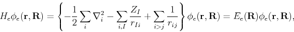
Using these facts, along with the electronic Schrdöinger equation,

$$\{T_e + {V}_{eN}({\bf r},{\bf R}) + {V}_{ee}\}\phi_e({\bf r},... ...) = {H}_e \phi_e({\bf r},{\bf R})= E_e \phi_e({\bf r},{\bf R})$$

we simplify Eq.(63) to

$$\phi_e({\bf r},{\bf R})T_N \phi_N({\bf R})+ \phi_N({\bf R})\phi_e({\bf r},{\bf R})(E_e + {V}_{NN})$$ (63)

$$- \left\{ \sum_A \frac{1}{2M} (2\nabla _R \phi_e({\bf r},{\b... ... + \phi_N({\bf R})\nabla^2_R \phi_e({\bf r},{\bf R})) \right\}$$ (64)

$$= E_{tot} \phi_e({\bf r},{\bf R})\phi_N({\bf R}).$$ (65)

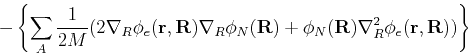
We must now estimate the magnitude of the last term in brackets. A typical contribution has the form $1/(2M) \nabla^2_R \phi_e({\bf r},{\bf R})$, but $\nabla _R \phi_e({\bf r},{\bf R})$ is of the same order as $\nabla_r \phi_e({\bf r},{\bf R})$ since the derivatives operate over approximately the same dimensions. The latter is $\phi_e({\bf r}, {\bf R}) p_e$, with $p_e$ the momentum of an electron. Therefore $1/(2M) \nabla^2_R \phi_e({\bf r},{\bf R})\approx p_e^2/(2M) = (m/M)E_e$. Since $m/M \sim 1/10000$, the term in brackets can be dropped, giving

$$\phi_e({\bf r},{\bf R})T_N \phi_N({\bf R})+ \phi_N({\bf R}) ... ...bf r},{\bf R})= E_{tot} \phi_e({\bf r},{\bf R})\phi_N({\bf R})$$

$$\{T_N + E_e + {V}_{NN} \} \phi_N({\bf R})= E_{tot} \phi_N({\bf R}).$$

This is the nuclear Shrödinger equation we anticipated-the nuclei move in a potential set up by the electrons.

To summarize, the large difference in the relative masses of the electrons and nuclei allows us to approximately separate the wavefunction as a product of nuclear and electronic terms. The electronic wavefucntion $\phi_e({\bf r},{\bf R})$ is solved for a given set of nuclear coordinates,

$${H}_e \phi_e({\bf r},{\bf R})= \left\{ -\frac{1}{2} \sum_i \... ...\phi_e({\bf r},{\bf R})= E_e({\bf R}) \phi_e({\bf r},{\bf R}),$$

and the electronic energy obtained contributes a potential term to the motion of the nuclei described by the nuclear wavefunction $\phi_N({\bf R})$.

$${H}_N \phi_N({\bf R})= \left\{ -\sum_I \frac{1}{2M_I} \nabla... ..._J}{R_{IJ}} \right\} \phi_N({\bf R})= E_{tot} \phi_N({\bf R})$$