Finite differences solution

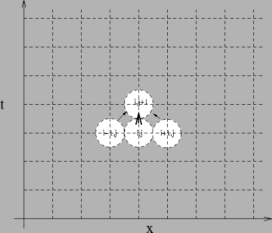
Figure 14: The finite differences algorithm for the heat equation.

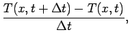
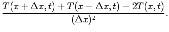
The numerical solution is based on converting the differential equation into an approximate finite-diffence one. Following a derivation similar to the one we used for the wave equation we approximate the derivatives by finite differences:

$$\frac{\partial T}{\partial t} = \frac{T(x,t+\Delta t)-T(x,t)}{\Delta t},$$ (69)

$$\frac{\partial^2 T}{\partial x^2} = \frac{T(x+\Delta x,t)+T(x-\Delta x,t)- 2T(x,t)}{(\Delta x)^2}.$$ (70)

Replacing in 66 we obtain the discrete equivalent:

$$T(x,t+\Delta t)=T(x,t)+\frac{\alpha}{C}\left[T(x+\delta x,t)+T(x-\Delta x,t) -2T(x,t) \right],$$ (71)

with the constant $C=(\Delta x)^2/\Delta t$. We see in Fig. 14 that the temperature at the point $(x, t+\Delta t)$ is determined by the temperatures at three points of the previous time step. The boundary conditions impose fixed values along the perimeter. The initial condition 67 is used to generate the temperature gradient at time $t=\Delta t$, and the equation is used for the time evolution.

The stability condition for a numerical solution is iven by

$$\alpha\frac{\Delta t}{(\Delta x)^2} \leq \frac{1}{4}.$$ (72)

This means that if we make the time step smaller we improve convergence, but if we decrease the space step without a simultaneous quadratic increase of the time step, we worsen it.