Exercise 6.1: Finite differences program

Solve the temperature distribution within an iron bar of length $l=50$cm with the boundary conditions

$$T(x=0,t)=T(x=l,t)=0,$$

and initial conditions

$$T(x,t=0)=100^{\circ}\mathrm{C}.$$

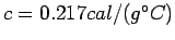
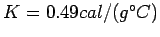
The corresponding constants for iron are:

$$c=0.113 \mathrm{cal/(g^{\circ} C)}, K=0.12 \mathrm{cal/(sg^{\circ}C)}, \rho=7.8 \mathrm{g/cc}.$$

1. Write the program to solve the heat flow equation using the finite differences method

2. Plot the temperature gradient along the bar at different instants of time. Use 100 space divissions for the calculation. Choose an appropiate time step such that the numerical solution is stable. Check that the temperature diverges with time is the constant $c$ is made larger that $0.5$.

3. Repeat the calculation for aluminum, $c=0.217cal/(g^{\circ}C)$, $K=0.49 cal/(g^{\circ}C)$, $\rho=2.7g/cc$. Note that the stability condition requires you to change the size of the time step.

4. Analize and compare the results for both materials. The shape of the curves may be the same but not the scale. Which bar cools faster and why?

5. Pick a sinusoidal initial gradient:
   
   $$T(x,t=0)=\sin{(\pi x/l)}.$$
   
   
   Compare with the analytic solution
   
   $$T(x,t)=\sin{(\frac{\pi x}{l})}e^{\pi^2\alpha t/l^2}.$$