Starting configuration

Figure 8: Initial configuration with particles in vertices of a a) triangular; b) rectangular lattice

Since the size of our system is typically 10-100 molecular diameters, this is certainly not a good representation for a macroscopic sample because most of the particles will be situated near a ``wall'' or ``boundary''. To minimize the effects of the boundaries and to simulate more closely the Since the size of our system is typically 10-100 molecular diameters, this is certainly not a good representation for a macroscopic sample because most of the particles will be situated near a ``wall'' or ``boundary''. 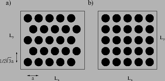To minimize the effects of the boundaries and to simulate more closely the Picking the right starting configuration is not trivial. The first choice would be to place the molecules randomly distributed, but this would give rice to large starting energies and forces, since many pairs would be placed at unphysical short distances. It is therefore customary to place the particles in the vertices of a some crystal lattice (face centered cubic -or triangular-, for instance). The $x$ and $y$ components of the velocities can be picked randomly in an interval $[-v_{\max },v_{\max }]$. Before starting the proper simulation and the measurement of the physical quantities, it is necessary to perform a ``thermalization'' run to let the system relax to a situation of dynamical and thermal equilibrium.