Exercise 12.3: MC simulation of the Ising model in 1D

1. Write a program to simulate the Ising model in the microcanonical ensemble in 1D. Use $N=100$, $J=1$, $h=0$, and a desired total energy $Eini=-20$. The physical quantities drift as the demon's energy is distributed over the $N$ spins. Compute a running average o the demon energy and $M$ as a function of the number of Monte Carlo steps per spin (our measure of ``time''). Note that the data is taken after every attempts rather than after every Monte Carlo step per spin. What is the approximate time necessary for these quantities to approach their equilibrium values? Modify the program so that you only start taking averages after some warmup time, leaving out the nonequilibrium configurations. What are the equilibrium values of $\langle E_d \rangle$, $\langle M \rangle$, and $\langle M^2 \rangle$? A choice of 1000 MC steps gives good results within $5\%$ accuracy.

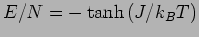
2. Use the relation (117) to obtain the equilibrium temperature $T$ for the system parameters considered in part 1. Measure $E$ in units of $J$. What is the corresponding energy of the system?

3. Compute $T$ and $E$ for the three cases $N=100$, $J=1$ and $Eini=-40, -60, -80$. Compare your results to the exact results for an infinite one-dimensional lattice $E/N=-\tanh{(J/k_BT)}$. How do your results for $E/N$ depend on the number of spins $N$ and the number of Monte Carlo steps per spin?

4. Use the same runs to compute $\langle M^2 \rangle$ as a function of $T$. Does $\langle M^2 \rangle$ increase or decrease with T?