Overview
This tutorial aims to discuss the manipulation of text in Excel. It seemed best to first discuss the functions in Excel available to manipulate strings and the strategies for handling the errors that may arise before getting into the examples that illustrate techniques and idioms.
- Description of the Excel Functions for Text Strings
IFand Conditional Expressions- Handling Errors
- Techniques and Idioms for Manipulating Text Strings
Description of the Excel Functions for Text Strings
For convenient reference, we first describle the Excel functions for text strings in a series of tables that group related functions. We will show the function name, how it is used, its purpose, and the conditions in which an error may occur. Specific examples of the use of these functions will be given in the section on Techniques and Idioms.
We will sprinkle some simple examples throughout this summary.
In these examples, we will assume that cell A1 has
the text:
Potter, Harry
and that cell A2 has the text:
Granger, Hermione
Excel views the characters within a text string as
numbered from position 1 up to its length.
In particular, positions outside this range are not valid.
The length may be computed by the function
LEN.
LEN |
LEN(text) |
Count of the characters in the text,
that is, its length.
|
|
If LEN is passed a cell reference or an entity
that has a valid representation as a string
(such as a number or the logical values
TRUE and FALSE),
then LEN
will return the length of the string representation of that
entity. Note, however, if the cell has special formatting
such as percent or currency, this will not be taken
into account in the computation of LEN on that
cell.
|
|
Error if
LEN is passed a cell reference or an entity
that evaluates to an error.
In that case, LEN
will return the same error.
|
| Example | Value | Comment |
LEN(A1) |
13 |
11 letters, 1 comma, 1 blank |
LEN(A2) |
17 |
15 letters, 1 comma, 1 blank |
The next operation shows that it is easy in Excel to join strings.
From a design point of view, this means that if you have a choice in
designing a spreadsheet then it is better to put separate components
of a string into separate cells and then join them if needed. On
the other hand, if text data is given to you as a lump then you may
need to split the data into chunks by the functions LEFT,
RIGHT, and MID.
CONCATENATE |
CONCATENATE(text1, text2, ...) |
Joins text1, text2, etc.,
to make a longer string
|
|
Shorthand: text1 & text2 & ... |
| Example | Value | Comment |
A1&"; "&A2 |
Potter, Harry; Granger, Hermione |
Join the strings with semicolon and blank in the middle |
The functions LEFT, RIGHT, and
MID are the tools for splitting text data into
chunks.
Notice that these functions require you to know exactly what
chunk of data is desired. To compute count and
start from the data itself, you may use the
search functions FIND and SEARCH.
LEFT |
LEFT(text,count) |
| Builds a string using the leftmost count characters of the text | |
Error if count < 0 |
|
If count = 0 then returns an empty string |
|
If count >= length then returns the entire string |
|
Idiom: To obtain the first character in a text string, use:
LEFT(text,1). |
|
RIGHT |
RIGHT(text,count) |
| Builds a string using the rightmost count characters of the text | |
Error if count < 0 |
|
If count = 0 then returns an empty string |
|
If count >= length then returns the entire string |
|
MID |
MID(text,start,count) |
| Builds a string starting at position start and using count characters of the text | |
Error if start <= 0 |
|
Error if count < 0 |
|
If count = 0 then returns an empty string |
|
If count >= (length - start)
then returns the rightmost portion of the string
that begins at start.
In particular, if you want the rightmost portion of a string that begins at start,
you may as well choose count to be
length.
|
|
Idiom: To obtain the character at position start
in a text string, use: MID(text,start,1). |
| Example | Value | Comment |
LEFT(A1,7) |
Potter, |
7 characters includes the comma |
LEFT(A1,6) |
Potter |
6 characters gets the last name: Potter |
LEFT(A2,8) |
Granger, |
8 characters includes the comma |
LEFT(A2,7) |
Granger |
7 characters gets the last name: Granger |
RIGHT(A1,5) |
Harry |
5 characters from the right gets the first name: Harry |
RIGHT(A2,8) |
Hermione |
8 characters from the right gets the first name: Hermione |
MID(A1,9,LEN(A1)) |
Harry |
First name, Harry, starts in position 9 and extends to end |
MID(A2,10,LEN(A2)) |
Hermione |
First name, Hermione, starts in position 10 and extends to end |
We now want to treat two problems of extracting text that cannot
be handled directly but must be handled via idioms. We will assume,
for ease of presentation, that the original string is in A1.
Problem 1: Extract the text from a given position start
to the end of a string.
The reason this problem requires an idiom is that both MID
and RIGHT require counts. Here are two idioms that solve
the problem.
    MID(A1,start,LEN(A1))

    RIGHT(A1,LEN(A1)-start+1)
The first idiom works as follows. The MID function is designed
to use start. Normally, it requires a precise count of how many
characters to extract. However, it is flexible and if it is given a count
that is “too big” then it will simply extract all characters from
start to the end of the string. Using LEN(A1) for
the count guarantees “too big”.
The second idiom computes how many characters to back up from the end of the
string to get back to and include start. The expression
LEN(A1)-start
will count only the characters from the end back to but not including
start itself. The extra +1 adds enough to include
the character at start.
Problem 2: Extract the text from a given position start
to a given position last in a string.
The idiom that solves this problem combines the reasoning of the two previous
idioms. You must use MID since you do not want all characters
to the right. You must also compute the count since now it must be exact.
Here is the solution.
MID(A1,start,last-start+1)
This idiom works since the number of characters to extract including both
start and last must be the difference
plus one.
The functions FIND and SEARCH permit
you to search for critical character positions within text data.
The search direction is from left to right. Unfortunately, Excel does not have built-in functions that search from right to left. Therefore, to search from right to left, you must somehow use the left to right functions to deliver the information that you need.
FIND |
FIND(search_text,text)
FIND(search_text,text,start)
|
FIND is case senstive |
|
| Searches for the search text within the text | |
| If found returns the character position where the search text begins | |
| The optional start parameter indicates where the search should start | |
| Error if the search text is not found | |
Error if start <= 0 |
|
SEARCH |
SEARCH(search_text,text)
SEARCH(search_text,text,start)
|
SEARCH is case insenstive |
|
| Searches for the search text within the text | |
| If found returns the character position where the search text begins | |
| The optional start parameter indicates where the search should start | |
| Error if the search text is not found | |
Error if start <= 0 |
| Example | Value | Comment |
FIND(", ",A1) |
7 |
Position of comma where comma-blank pair matches |
FIND(", ",A2) |
8 |
Position of comma where comma-blank pair matches |
FIND("T",A1) |
#VALUE! |
Error: FIND is case sensitive and "T" is not in the text |
SEARCH("T",A1) |
3 |
SEARCH is case insensitive and "T" matches "t" in position 3 |
FIND("n",A2) |
4 |
The first "n" is in position 4 |
FIND("n",A2,5) |
16 |
The first "n" in position 5 or later is in position 16 |
The functions TRIM and CLEAN
tidy up text.
TRIM |
TRIM(text) |
| Removes leading and trailing spaces and converts any sequence of internal spaces to a single space. | |
CLEAN |
CLEAN(text) |
|
Removes non-viewable characters from the text.
This is useful primarily if the text was imported from an external source that embeds characters that cannot be viewed. |
The function SUBSTITUTE permits the subsitution
of new text for old text within a larger text string.
SUBSTITUTE |
SUBSTITUTE(text, old_text, new_text)
SUBSTITUTE(text, old_text, new_text, occurence)
|
SUBSTITUTE
is case senstive in its matching |
|
| Makes replacements in the given text of exact matches of the old text with the new text. | |
If the optional parameter occurence is missing
then replaces all exact matches of the old text with
the new text.
|
|
If the optional parameter occurence is present
then looks for that particular occurence of the old text
and replaces only that occurence with the new text.
|
|
Error if occurence <= 0 |
| Example | Value | Comment |
SUBSTITUTE(A1,"o","a") |
Patter, Harry |
Replace all "o" with "a" |
SUBSTITUTE(A1,"a","o") |
Potter, Horry |
Replace all "a" with "o" |
SUBSTITUTE(A2,"G","St") |
Stranger, Hermione |
Replace all "G" with "St" |
SUBSTITUTE(A1,"r","d") |
Potted, Haddy |
Replace all "r" with "d" |
SUBSTITUTE(A1,"r","d",1) |
Potted, Harry |
Replace occurence #1 of "r" with "d" |
SUBSTITUTE(A1,"r","d",3) |
Potter, Hardy |
Replace occurence #3 of "r" with "d" |
There are two utility functions CHAR and CODE
that are occasionally useful.
CHAR |
CHAR(number) |
Constructs a string of length 1 corresponding to
the given number which represents a character code.
|
|
Error of type #VALUE!
if number <= 0 or number >= 256.
|
|
The test spreadsheet
characters.xls
may be used to show which characters will be represented on a
particular machine and operating system.
If you compare characters.xls on a PC and Macintosh,
you will see that there is agreement on the characters with codes
from 32 to 126. Otherwise you will
mostly see differences. For an in-depth explanation together
with screen snapsnots of the characters represented, see the
Discussion below.
|
|
The blank or space character has code 32. |
|
The digit characters 0 ... 9 have consecutive codes
48 ... 57.
|
|
The upper case letters A ... Z have consecutive codes
65 ... 90.
|
|
The lower case letters a ... z have consecutive codes
97 ... 122.
|
|
All other characters in the code range from 32 to
126 represent common punctuation marks.
|
|
| It is possible to use the consecutive aspect of the codes for
the upper and lower case letters to generate a sequence of such
letters in a spreadsheet via formulas.
See Techniques and Idioms below. |
|
| Discussion | |
CODE |
CODE(text) |
| Returns the character code of the first character in the text string. | |
If CODE is passed a cell reference or an entity
that has a valid representation as a string
(such as a number or the logical values
TRUE and FALSE),
then CODE
will return the character code of the first character in
the string representation of that
entity. Note, however, if the cell has special formatting
such as percent or currency, this will not be taken
into account in the computation of the first character code.
|
|
Error if CODE is
passed an entity that corresponds to an empty
string.
A string with 0 characters is considered
empty.
A string with one blank character is not considered empty even though you cannot see this blank on the screen. |
Discussion of Character Codes
The characters represented in Excel are based in part on international standards and in part on decisions specific to a machine or operating system. To understand this better, it is useful to consider a division of the characters in two different ways.
-
The division into code pages.
Code Page 0 is the range of codes from
0to127.Code Page 1 is the range of codes from128to255. -
The division of character codes into printable characters
and control codes.
The control codes are
0 ... 31, 127, ... 159, 173.
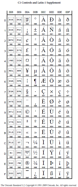
To make this concrete, let us immediately show screen snapshots of
code pages 0 and 1 from the
Unicode
international standard and from the characters actually displayed
on a PC and Macintosh using the test spreadsheet
characters.xls.
| Source | Code Page 0 | Code Page 1 |
|---|---|---|
| Unicode | 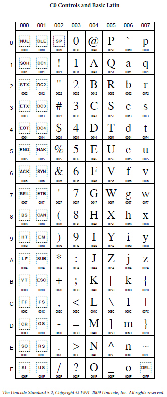 |
 |
| PC | 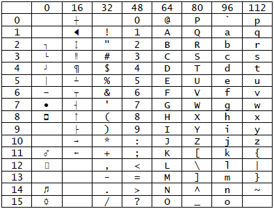 |
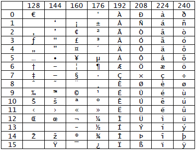 |
| Mac | 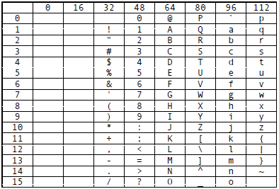 |
 |
In the table above, the PC and Mac screen snapshots are at 50% of full size. If you wish to view the character data at full size or if you wish to print the character data, click on the link character table.
Now let us resume the discussion.
The design of Code Page 0 originated in the 1960’s on the
American Standard Code for Information Interchange known as
ASCII. The history is described in a Wikipedia article on
ASCII.
The key points of this design were that digits, uppercase letters, and
lowercase letters form three sequences without interruption. This was
not the case in more primitive character sets and was quite inconvenient.
Furthermore, internally in ASCII, a matching pair of uppercase and
lowercase characters differ in a single bit which makes case insensitive
sorting and searching easy to implement. Finally, control codes
were grouped into two blocks 0 ... 31 and the single
character in position 127 that corresponds to forward delete.
The control codes in 0 ... 31 include tab, line feed,
carriage return, and backward delete, together with many esoteric control
codes. The blank or space was set into position 32 so it
would be the first printable character and would therefore “sort
first” in any sorting operation.
As you can see from the above snapshot of the Unicode Code Page 0 the decisions from the ASCII standard have been carried forward into Unicode.
It was not originally intended that control codes should be printable. However, in the original IBM PC, printable representations of some control codes were introduced and these appear in the PC table for Code Page 0. As you can see, the Macintosh sticks to the original design that the control codes in Code Page 0 have no printable representation.
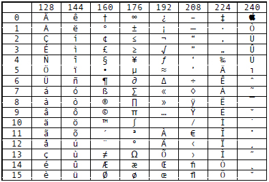
Code Page 1 was not initially standardized and therefore the situation emerged that each manufacturer could do as they wished. Since Apple wanted to support European alphabets in the Macintosh, they designed a version of Code Page 1 with many accented characters, some additional punctuation, and a few mathemathematical symbols. In its time, this was a real advance.
The goal of Unicode
is to design a code system to capture all the alphabets of the world.
In implementing this goal,
the decision was made to follow a different path than the Macintosh. The
result was the version of Code Page 1 that you see above. One design
decision was to introduce 32 additional control codes in the range
128 ... 159 parallel to the earlier control codes in the range
0 ... 31. There was also one further control code placed in
the strange position 173.
The remaining characters in the Unicode
Code Page 1 are printable and many of them correspond to characters in
the Macintosh set but are in entirely different positions. This leads to
unfortunate incompatibility. Unicode has a special character in position
160 called non-breaking-space or NBSP. This space
is the same width as an ordinary space but it signals to software that the
text connected by this type of space should never be split at a line break.
This turns out to important for formatting especially on the web.
The printable characters in the PC Code Page 1 are identical to the corresponding characters in the Unicode Code Page 1. However, unlike Unicode, the PC continues its tradition of giving printable representations to many of the control codes as well.
The bottom line for users of Excel is that if you want to build a spreadsheet
that may be viewed correctly on both a PC and a Mac then you must stick to the
characters on Code Page 0 in positions 32 ... 126.
If as an Excel user you are willing to forego Mac compatibility but you wish to retain Unicode compatibility, then stick to the Unicode printable characters.
If as an Excel user you can guarantee that your users will run your spreadsheet only on a PC running Windows then you may use all of the PC characters.
The only exception to these recommendations is Line Feed or character
10 which is the topic of the next section.
The Line Feed Character CHAR(10),
Alt-Enter, and the Wrap Text Property
There is one control character line feed or
CHAR(10) that deserves further discussion.
Sometimes when you enter data into a cell, you may wish the data to occupy two or more lines within that cell. Excel offers a keyboard shortcut alt-Enter to insert a line feed within the cell. Characters that follow the line feed will be on a new line.
The use of alt-Enter actually performs 2 tasks:
-
The line feed character
CHAR(10)is added to the string being constructed in the cell. - The cell property Wrap Text is turned on for the cell so that multiple lines can be displayed.
You may ask whether it is possible to use Excel formulas to
cause text in a cell to have line breaks. Unfortunately,
the answer is no. It is easy to insert CHAR(10)
into a string of text but there is no way to use formulas to
turn on the Wrap Text property of a cell. This is
because formulas compute the values to be placed in the cell
but cannot be used to set the cell formatting properties.
This situation is illustrated in the following screen snapshot:
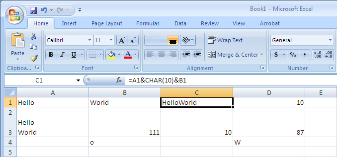
In row 1, the text Hello and World
has been placed in cells A1 and B1. In cell
C1, we have used the concatenation operator &
to join these two text segments with one CHAR(10) in the
middle. As you can see, the text is still shown on one line and there
is no visible indication of presence of the CHAR(10). On
the other hand, cell D1 uses the formula
=CODE(MID(C1,6,1)) to find the character code of the 6th
character in the cell C1 and sure enough the code is
10 as it should be. Therefore the line feed is present
in cell C1 but it is invisible.
In cell A3, we have used alt-Enter. Specifically,
we have typed the following 11 characters:
H e l l o alt-Enter W o r l d
As soon as alt-Enter is typed, Excel turns on the Wrap Text property for the cell so the text will show multiple lines. Alas, there is no way using functions to accomplish the same trick.
If we test the contents of cells A3 and C1 for
equality, it will turn out that the contents are equal. The difference
is simply a matter of the Wrap Text property.
The Wrap Text property may be turned on for an individual cell
(such as cell C1) or for a selection of cells
by clicking on the Wrap Text command in the
Excel ribbon at the top of the window:

Normally, wrapping text is useful only in particular cells so it is usually turned only as needed.
Transforms to Upper, Lower, or Proper Case
UPPER |
UPPER(text) |
| Returns a string with all alphabetic characters capitalized, that is, converted to upper case. | |
LOWER |
LOWER(text) |
| Returns a string with all alphabetic characters converted to lower case. | |
PROPER |
PROPER(text) |
|
Returns a string with alphabetic characters
capitalized as follows.
The first character in each word is capitalized and all other characters are converted to lower case. |
Conversion of Numbers to Text or Text to Numbers
TEXT |
TEXT(number, format_string) |
| The number is converted to a text string using an Excel custom number format string. The full details on formats may be found by searching Excel Help for the italicized phrase above. | |
FIXED |
FIXED(number)
FIXED(number, decimal_places)
FIXED(number, decimal_places, no_commas)
|
|
The number is converted to text according to the following
rules.
Rounds the number to the given decimal_places
if provided or to 2 decimal places if the parameter is omitted.
By default, commas are inserted for every 3 digits. To eliminate commas, no_commas must be
provided and must be TRUE.
|
|
If decimal_places < 0, this function will round
to multiples of 10, or 100, or 1000, or whatever depending on
the precise negative value of decimal_places.
|
|
DOLLAR |
DOLLAR(number)
DOLLAR(number, decimal_places)
|
|
The number is converted to currency formatted text according to
the following rules.
Rounds the number to the given decimal_places
if provided or to 2 decimal places if the parameter is omitted.
|
|
If decimal_places < 0, this function will round
to multiples of 10, or 100, or 1000, or whatever depending on
the precise negative value of decimal_places.
|
|
VALUE |
VALUE(text) |
| Converts the text to a number provided that Excel can interpret the text as the representation of a number. | |
| Error if the text is not a valid representation of a number. In particular, extra non-numeric characters in the text will cause this function to return an error. |
Final Note
There are a small number of additional text functions, namely,
EXACT,
REPT,
T,
N.
Since these are rarely used, we refer you to Excel Help
for more information.
IF and Conditional Expressions
Excel has an extremely powerful function IF
that will return one of two choices depending on the
value of a condition parameter.
IF |
IF(condition, expression-1, expression-2) |
In the most common cases, condition is an expression
that evaluates to TRUE or FALSE.
If condition is TRUE,
then the function returns the value of expression-1.
If condition is FALSE,
then the function returns the value of expression-2.
|
|
Excel will also accept a number for the condition.
In that case, a non-zero number acts a TRUE while
zero acts as FALSE.
|
|
Error if the condition
is none of TRUE, FALSE, or a number.
|
|
| Error if the evaluation of the condition or the expression chosen results in an error. |
Let us now summarize the important ways that a TRUE or
FALSE expression may be formed aside from the trivial
act of embedding these values as constants.
The first mechanism is to compare two entities for equals, not equals, or various forms of inequality comparison. This is done using one of six operators listed in the table.
| op | |
= |
Equals |
<> |
Not equals |
< |
Less than |
<= |
Less than or equals |
> |
Greater than |
>= |
Greater than or equals |
Generally, a comparision operation has the form
entity-1 op entity-2
where op is one of the 6 operators in the table.
Any two entities may be compared with = or
<>. The other operators may be used
only when the comparison makes sense.
For example, the expression A1 > 0 tests
if cell A1 has a numeric value and is
greater than zero.
Next, there are test functions that directly return
TRUE or FALSE when given an
expression to examine.
IS... Functions |
IS...(expression) |
ISBLANK |
Is empty, that is, has no content |
ISTEXT |
Is text and is not blank |
ISNONTEXT |
Is anything except text-that-is-not-blank |
ISNUMBER |
Is a number and is not blank |
ISEVEN |
Is an even number |
ISODD |
Is an odd number |
ISLOGICAL |
Is TRUE or FALSE |
ISREF |
Is a cell reference |
ISERROR |
Is an error state |
ISNA |
Is the specific error state #N/A |
ISERR |
Is an error state but is not #N/A |
An interesting question is: What happens if you type the
characters true into a cell. Is the result
LOGICAL or TEXT or both?
The answer is that Excel will convert what you have just
typed into TRUE and center it in the cell.
Further, ISLOGICAL will return
TRUE while
ISTEXT will return FALSE.
In particular, to enter true as TEXT, you
must enter it in quoted form 'true.
Then, ISLOGICAL will return
FALSE while
ISTEXT will return TRUE.
Now that we have seen how to create simple TRUE/FALSE
results using operators and the IS... functions,
let us describe the 3 Excel functions
designed to manipulate and combine
logical conditions into compound logical conditions.
AND |
AND(condition-1,condition-2,...) |
Returns TRUE if all conditions evaluate
to TRUE.
Returns FALSE if any single condition
returns FALSE.
|
|
| Error if the evaluation of any condition results in an error. | |
OR |
OR(condition-1,condition-2,...) |
Returns TRUE if any single condition
returns TRUE.
Returns FALSE if all conditions evaluate
to FALSE.
|
|
| Error if the evaluation of any condition results in an error. | |
NOT |
NOT(condition) |
|
Reverses the value of the condition.
If the condition is TRUE then returns FALSE.
If the condition is FALSE then returns TRUE.
|
|
| Error if the evaluation of the condition results in an error. |
Using simple conditions together with the power of combinations provided by
AND, OR, and NOT,
you can make extremely precise
statements about when some action should or should not take place.
Feeding simple or compound conditions into the IF function
will give you the power to determine precisely what is evaluated for any
particular cell. In turn, this leads to the power to control the behavior
of the entire spreadsheet.
Let us give some examples of IF using an exam grade as the
topic. Let us assume the exam grade is in cell A1 and
we wish to give verbal feedback in cell B1.
To start simply, suppose that if the grade is 90 or above,
we want the feedback to be Excellent!, and if the grade is
less then the feedback will be blank. We can do this with the
following formula in B1:
=IF(A1>=90,"Excellent!","")
Of course, it would be nice to give better feedback for the grades
below 90 as well.
To do this using IF requires using nested
IF statements. To make it easy to see what is going
on, I will write the formula on this web page vertically, but keep
in mind that in Excel the formula would need to be on one line.
    =IF(A1>=90,"Excellent!",
        IF(A1>=80,"Good",
        IF(A1>=60,"Fair",
        IF(A1>=50,"Dismal but passing","Utter failure"))))
This formula gives distinct feedback for grades above 90, grades in the range 80-89, grades in the range 60-79, grades in the range 50-59, and finally grades below 50.
The formula also illustrates the zen of nested IF
statements. The first expression after the condition tells what you
want if the condition is TRUE while the second expression
after the condition starts another IF to test another
condition and continue. Notice that this pattern holds until the last
where you simply respond with Utter failure.
Sometimes, one can replace nested IF's by using one of
the functions VLOOKUP or HLOOKUP. We will
not attempt to discuss this alternative here.
Handling Errors
In the previous section, we listed three functions that detect the presence of an error.
ISERROR |
Is an error state |
ISNA |
Is the specific error state #N/A |
ISERR |
Is an error state but is not #N/A |
Normally, to check for an error, we recommend using the function
ISERROR. Let us briefly explain why.
Excel has a special function NA() that allows a
spreadsheet designer to intentionally insert the #N/A
error to signal some special problem. In that case, other code
that needs to check for errors may need to distinguish between
the #N/A error and all other errors. In normal
usage, however, this degree of subtlety is quite unnecessary.
So now let us consider the general scenario for using
ISERROR for error testing. Let's assume:
-
We wish to test an
expressionfor an error. -
We wish to use
alternativeif there is an error. -
We wish to use
firstchoiceif everything is fine.
Then, from a structural point of view, here is the code using an
IF together with ISERROR:
IF(ISERROR(expression),alternative,firstchoice)
Often, of course, the firstchoice is precisely the
expression that you are testing for an error. In
this common case, the above structure becomes:
IF(ISERROR(expression),alternative,expression)
In other words, if you have an error use the alternative,
otherwise use the expression.
Although this structure is absolutely correct, it is also annoying
because expression must be typed into the formula twice
and must be evaluated twice when the IF is evaluated.
To avoid this annoyance, Excel has a special test IFERROR
that permits you to type
expression and alternative once each:
IFERROR(expression,alternative)
IFERROR works as follows. If expression does
not result in an error then it’s value is returned. If
expression does produce an error then
alternative is returned.
IFERROR will be illustrated in the section on
Techniques and Idioms.
Esoteric Details about Types and Errors in Excel
It is possible to drill more deeply using the functions
TYPE and ERROR.TYPE.
The function TYPE returns the type of the value
of an expression but does not say whether that value was
directly given or is the result of a formula. This function
returns one of 5 codes:
1corresponds to a number or a blank2corresponds to a text value4corresponds to a logical value16corresponds to an error64corresponds to an array or range
The function ERROR.TYPE (notice the period) returns
one of 8 codes that can better explain an error in an expression
that contains an error:
1corresponds to#NULL!:
Incorrect range separator or range intersection2corresponds to#DIV/0!:
Division by zero3corresponds to#VALUE!:
A parameter value to a function has the wrong type4corresponds to#REF!:
Reference to cells with no data or that do not exist5corresponds to#NAME?:
Reference to names that do not exist (ranges, functions, ...)
May be due to failure to quote a string parameter6corresponds to#NUM!:
Passing an incorrect argument to a function or returning a numeric value that is too big or too small to represent7corresponds to#N/A:
Something is not available (lookup match, worksheet function, required parameters to a function, ...)8corresponds to#GETTING_DATA
Techniques and Idioms for Manipulating Text Strings
The examples in this section may be found in the spreadsheet
strings.xlsx.
The xlsx format was chosen because Excel issued a warning
that some function used in this spreadsheet did not exist when the
older xls format was designed. The spreadsheet will
download with no problems using Firefox. However, Internet Explorer
has a bug and will change the file extension from xlsx to
zip. This must be fixed by hand. In the first dialog
box, choose Save. In the second dialog box, change
Winzip Files in the dropdown to All Files
and then manually replace the extension zip with the
extension xlsx. This bug is quite annoying since both
IE and Excel are Microsoft products and you would think they would
work together better.
Example: Generating the letters A to Z in a column
In Excel, it is easy to generate a column of numbers 1 2 3 ....
We will see that it is almost as easy to generate a column of letters.
To generate 1 2 3 ... starting in cell A3, we
enter the constant 1 into A3 and the formula
=A3+1 into the cell below A4. This places
2 into A4 and provides the relative formula
that may be dragged downwards to generate the additional numbers.
To generate A B C ... starting in cell B3, we
must be a bit more sophisticated since we cannot simply add 1 to
a letter. However, we can add 1 to a character code and
make use of the fact that the upper case letters have consecutive
character codes. The process is this:
-
Use
CODEto convert a letter to its character code. - Add 1 to the character code
-
Use
CHARto convert the new character code to a letter.
The details of the process are shown in the snapshot below where the
cell formulas in the B column are typed as text in the
C column.
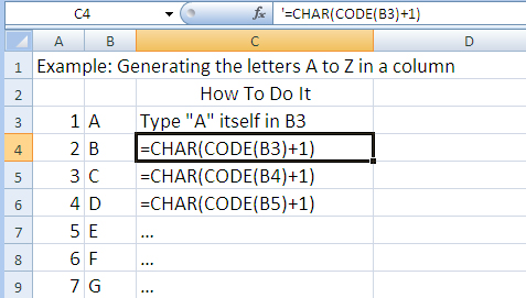
The process is seeded by typing A into cell B3.
Then to fill B4 we proceed as follows:
The character code of cell B3 is computed as
CODE(B3)
Add 1 to this to get CODE(B3)+1
Insert the new character into cell B4 via
=CHAR(CODE(B3)+1)
The formula in cell B4 is now a properly relative formula
that may be dragged downward to generate the rest of the upper case
letters.
Example: Parsing Presidential Names
Parsing is the process of breaking a text string into pieces based on a desired set of goals. This example will illustrate such a process using a list with some of the names of US presidents.
The list of presidential names is given in column A of
the spreadsheet shown in the snapshot below.
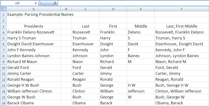
Notice that in some cases there is only a first and last name; in other cases there is a full middle name; and in other cases there are one or two middle initials.
The parsing problem is to break up each name into the Last
name, First name, and Middle name or initials if
any. Under no circumstances should an error show up on the
spreadsheet. You can see in the snapshot that this problem is
solved in columns C, D, and
E.
A related recombination problem is to present the same data in the form:
Last, First Middle
This problem is solved in column F. As you will
see, the recombination problem is easy once the
parsing problem is solved.
One key to solving a parsing problem is to know what assumptions you may count on. This allows you to know when error checking may be needed and when it may be skipped. Our assumptions are:
- Each presidential name is given in the order First Middle Last with only blank separators.
- There are no leading or trailing blanks and no run of two blanks in a row in the inner part of the text.
- Each string has at least one blank and at most three blanks.
In this parsing problem, the key will be to find the blanks
since the blanks are the separators between the segments of text
that we wish. Recall from the discussion of
String Functions that the two functions
FIND and SEARCH both search from left to
right and that there is no built-in function to search from right
to left. We will soon need to deal with this limitation.
We will describe the creation of the formulas by focusing on row
4. The formulas will then drag downwards to solve
the problem in general.
Since the First name is at the left, this is the easiest segment of text to find. Furthermore, since we know that at least one blank occurs in the string, we know that the following search for the first blank must succeed:
FIND(" ",A4)
The first blank is one character after the end of the First name. Hence the position of the last character in First name is given by the expression:
FIND(" ",A4)-1
To make it easy to check for correctness, we will store this
value in cell G4. We will also label column
G with Before1 to indicate that it holds
the last position before the 1st blank. Column G
is our first helper column.
Using the LEFT function, we can now extract
the First name by the formula:
=LEFT(A4,G4)
This formula is placed in cell D4.
The Middle names are the most difficult to handle because some are missing, some have a full name, some have one initial, one has two initials. Therefore, we first focus on finding the Last name. The principle we will use is this:
The start character of the Last name is the first character after the rightmost blank in the string.
This principle is great except that we do not know if there are one,
two, or three blanks in a particular string. If we search for a
blank that is not there, we must use IFERROR to handle
the error.
Our strategy is illustrated in the next snapshot.
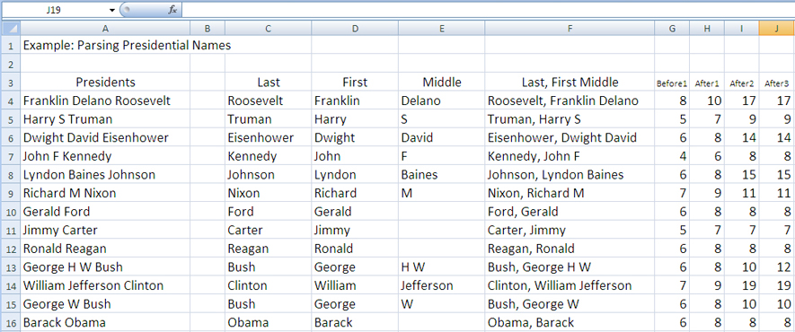
We create three additional helper columns labeled After1, After2, and After3. Here is how these three columns are defined conceptually.
- After1 is the position after the first blank which we know must exist.
- After2 is the position after the second blank if that exists or is equal to After1 otherwise.
- After3 is the position after the third blank if that exists or is equal to After2 otherwise.
If you examine the numerical data in the snapshot above and compare that data with the presidental names, you will see that the numerical data does indeed meet the conditions specified. We will now explain how these numerical values are computed.
Since the first blank must exist, we can compute the After1
cell H4 with the formula:
=FIND(" ",A4)+1
To proceed forward, the key insight is that we must search for
the possible second blank starting with the value in the column
After1. If we were certain that a second blank existed,
we could use the following formula in cell I4 that
uses the value in cell H4 as the start position:
=FIND(" ",A4,H4)+1
However, a second blank may not exist, so we must use
IFERROR to construct the formula for cell
I4 in column After2:
=IFERROR(FIND(" ",A4,H4)+1,H4)
This formula says to use the computation for the second blank
if it works and otherwise to use the value already in
cell H4 in column After1.
The formula for the possible third blank is obtained in the
same way. In cell J4 of column After3,
we place the formula:
=IFERROR(FIND(" ",A4,I4)+1,I4)
The net effect of this technique is that After3 must contain the position that is one character after the rightmost blank, that is, the start position of the Last name.
We can therefore use the MID function to extract
the Last name. To do this, we put the following
formula in cell C4:
=MID(A4,J4,LEN(A4))
This formula says to go to the string in cell A4,
use the start position in cell J4, and extract
as many characters as possible. Note that MID
does not care if the count specified in the third parameter
is too big so we just use LEN(A4) which is
enough.
Finally, we go back to the question of Middle. We
first observe that column After1 contains the start
position of Middle since it is the position of the
first character after the first blank. We also know that
we need to grab characters up to but not including the
position in After3 and that if we do so we may need
to deal with one trailing blank. To accomplish this, we
combine MID with TRIM and place the
following formula in cell E4:
=TRIM(MID(A4,H4,J4-H4))
This formula says to grab all possible characters in Middle and then to trim to remove the trailing blank. Notice that this approach utterly sidesteps the question of whether Middle exists, is a full name, or is one or two initials. It is very pleasing when you can solve a tricky problem by working around it.
As we said at the start of this section, the recombination
problem is easy using concatenation. We simply put the following
formula into cell F4 using the concatenation operator
&:
=C4&", "&D4&" "&E4
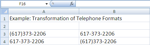
Example: Transformation of Telephone Formats
This section illustrates the use of SUBSTITUTE to
transform the format of a US telephone number. In the snapshot
below, the text in column B has been transformed
from the original text in column A. You will see
that the transform in row 4 reverses the transform
in row 3.
Since this example is actually quite simple, we will simply
give the formulas used in cells B3 and
B4 with brief comments.
In B3:
=SUBSTITUTE(SUBSTITUTE(A3,")","-"),"(","")
The inner SUBSTITUTE replaces the right
parenthesis with a hyphen while
the outer SUBSTITUTE replaces the left
parenthesis with an empty string.
In B4:
="("&SUBSTITUTE(A4,"-",")",1)
A left parenthesis is concatenated on the front of the string and the first occurrence of a hyphen is replaced by a right parenthesis.