The Ising model

Consider a lattice with $N$ sites, where each site $i$ can assume two possible states $s_i=+1,-1$, or spin ``up'' and spin ``down''. A particular configuration or microstate of the lattice is specified by the set of variables $\{s_1,s_2,...s_N\}$ for all lattice sites.

Now we need to know the dependence of the energy $E$ of a given microstate, according to the configuration of spins. The total energy in the presence of a uniform magnetic field is given by the ``Ising model'':

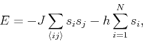$$E=-J\sum_{\langle ij \rangle}s_is_j-h\sum_{i=1}^Ns_i,$$ (276)

where the first summation is over all nearest neighbor pairs and the second summation is over all the spins of the lattice. The ``exchange constant'' $J$ is a measure of the strength of the interaction between nearest neighbor spins. If $J>0$, the states with the spins aligned $\uparrow \uparrow$ and $\downarrow \downarrow$ are energetically favored, while for $J<0$ the configurations with the spins antiparallel $\uparrow downarrow$ and $\downarrow \uparrow$ are the ones that are preferred. In the first case, we expect that the state with lower energy is ``ferromagnetic'', while in the second case, we expect it to be ``antiferromagnetic''. If we subject the system to a uniform magnetic field $h$ directed upward, the spins $\uparrow$ and $\downarrow$ possess and additional energy $-h$ and $+h$ respectively. Note that we chose the units of $h$ such that the magnetic moment per spin is unity.

Instead of obeying Newton's laws, the dynamics of the Ising model corresponds to ``spin flip'' processes: a spin is chosen randomly, and the trial change corresponds to a flip of the spin $\uparrow \rightarrow \downarrow$ or $\downarrow \rightarrow \uparrow$.