General case: Linear Combination of Atomic Orbitals

Let us consider a more general case, independently of the form of the Hamiltonian and the crystal structure. We are assuming for simplicity that we have one atom per unit cell (we shall see the generalization later), and the electron-electron interarctions are ignored.

We shall write the wave function for a single site, as a linear combinatioj of atomic orbitals

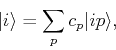$$\vert i\rangle = \sum_p c_p \vert ip\rangle,$$ (186)

wheer the coefficient $c_i$ are unknown. We are also assuming that the different orbitals form a locally orthogonal basis:

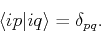$$\langle ip\vert iq\rangle = \delta_{pq}.$$ (187)

This does not mean that the orbitals on different sites will not have a finite overlap. Let us write a $k$-state as:

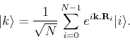$$\vert k\rangle = \frac{1}{\sqrt{N}} \sum_{i=0}^{N-1} e^{i{\bf k}.{\bf R}_i} \vert i\rangle.$$ (188)

We want to explicitly obtain a form for the eigenvalue equation

$$H\vert k\rangle = \epsilon(k)\vert k\rangle.$$ (189)

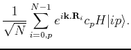
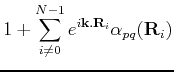
Applying the Hamiltonian on the state $\vert k\rangle$ yields:

$$H\vert k\rangle = \frac{1}{\sqrt{N}} \sum_{i=0,p}^{N-1} e^{i{\bf k}.{\bf R}_i} c_p H\vert ip\rangle.$$ (190)

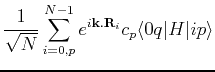
We now multiply from the left by $\vertq\rangle$, to obtain

$$\langle 0q\vert H\vert k\rangle = \frac{1}{\sqrt{N}} \sum_{i=0,p}^{N-1} e^{i{\bf k}.{\bf R}_i} c_p \langle 0q\vert H\vert ip\rangle$$ (191)

$$= \epsilon(k) \sum_{i=0,p}^{N-1} e^{i{\bf k}.{\bf R}_i} c_p \langle 0q\vert ip\rangle.$$ (192)

This leads to a generalized eigenvalue equation of the form

$$HC(k) = \epsilon(k) S C(k)$$ (193)

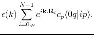
in order to calculate the matrix elements explicitly, let us break $H$ into a pice containing the atomic potential on site $0$, $H_{at}$, and the remaning part in a term that we call $\Delta U$. Therefore, we obtain:

$$\langle 0p\vert H\vertq\rangle = \langle 0p\vert H_{at}\vertq\rangle = \epsilon_p \delta_{pq}$$ (194)

$$\langle 0p\vert H\vertq\rangle = \langle 0p\vert\Delta U \vert iq\rangle = \gamma_{pq}({\bf R}_i)$$ (195)

$$\langle 0p\vert iq \rangle = \alpha_{pq}({\bf R}_i)$$ (196)

this yields

$$H_{pq} = \sum_{i \neq 0}^{N-1} e^{i{\bf k}.{\bf R}_i} \gamma_{pq}({\bf R}_i) + \epsilon_p \delta_{pq}$$ (197)

$$S_{pq} = 1+ \sum_{i\neq0}^{N-1} e^{i{\bf k}.{\bf R}_i} \alpha_{pq}({\bf R}_i)$$ (198)