


Next: Projector Monte Carlo
Up: Quantum Monte Carlo
Previous: Measurement and averaging
In this section, we will briefly describe an application of this general
algorithm to the quantum mechanical many-body problem of interacting
electrons on a lattice, working in the grand-canonical ensemble. The basic
idea of this approach was presented some time ago by Blankenbecler,
Scalapino and Sugar. [13]
Quantum Monte Carlo relies on the fact that  -dimensional quantum problems
can be intepreted as classical problems in
-dimensional quantum problems
can be intepreted as classical problems in  dimensions through
Feymann's Path Integral representation. The task consists in identifying
Ising-like fields that would allow us to evaluate the partition function and
mean values using the same Metropolis algorithm we have used before in the
equivalent classical model. Suzuki [14] was the first to apply this
concepts after generalizing an idea by Trotter. [15]
dimensions through
Feymann's Path Integral representation. The task consists in identifying
Ising-like fields that would allow us to evaluate the partition function and
mean values using the same Metropolis algorithm we have used before in the
equivalent classical model. Suzuki [14] was the first to apply this
concepts after generalizing an idea by Trotter. [15]
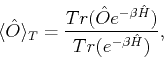
Suppose we want to evaluate the expectation value of a physical observable  , at some finite temperature
  . If
. If  is the
Hamiltonian of the model, this expectation value is defined as,
is the
Hamiltonian of the model, this expectation value is defined as,
 |
(307) |
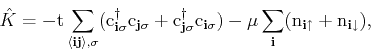
where the notation is the standard. From now on, let us
concentrate on the particular case of the one band Hubbard model which was
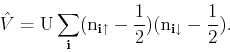
defined previously. The Hamiltonian of this model, with the addition of a
chemical potential, can be naturally separated into two terms as,
 |
(308) |
 |
(309) |
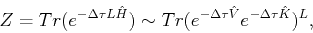
Discretizing the inverse temperature interval as
 , where
  is a small number, and
  is the total number
of time slices, we can apply the well-known Trotter's formula to rewrite the
partition function as,
is the total number
of time slices, we can apply the well-known Trotter's formula to rewrite the
partition function as,
 |
(310) |
where a systematic error of order
 has been
introduced, since
has been
introduced, since
![$[{\hat{K}},{\hat{V}}]\neq 0$](img971.png) . In order to integrate out
the fermionic fields the interaction term
. In order to integrate out
the fermionic fields the interaction term  has to be made
quadratic in the fermionic creation and annihilation operators by
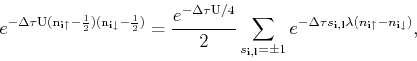
introducing a decoupling Hubbard-Stratonovich transformation. At this stage,
we can select from a wide variety of possibilities to carry out this
decoupling i.e. we can choose continuous or discrete, real or complex
fields, belonging to different groups. In particular, and for illustration
purposes, here we use a simple transformation using a discrete ``spin-like''
field [16],
has to be made
quadratic in the fermionic creation and annihilation operators by
introducing a decoupling Hubbard-Stratonovich transformation. At this stage,
we can select from a wide variety of possibilities to carry out this
decoupling i.e. we can choose continuous or discrete, real or complex
fields, belonging to different groups. In particular, and for illustration
purposes, here we use a simple transformation using a discrete ``spin-like''
field [16],
 |
(311) |
which is carried out at each lattice site  , and for
each temperature (or imaginary-time) slice
, and for
each temperature (or imaginary-time) slice  . The constant
  is
defined through the relation
is
defined through the relation
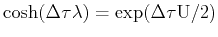 . The transformation Eq.(314) reduces the four-fermion
self-interaction of the Hubbard model to a quadratic term in the fermions
coupled to the new spin-like field
. The transformation Eq.(314) reduces the four-fermion
self-interaction of the Hubbard model to a quadratic term in the fermions
coupled to the new spin-like field
 . Thus, in this
formalism the interactions between electrons are mediated by the spin field.
Now we can carry out the integration of the fermions. While this is
conceptually straightforward, and for a finite lattice of
. Thus, in this
formalism the interactions between electrons are mediated by the spin field.
Now we can carry out the integration of the fermions. While this is
conceptually straightforward, and for a finite lattice of
 sites it gives determinants of well-defined matrices, arriving
to the actual form of these matrices is somewhat involved, and beyond the
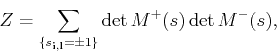
scope of this review. Then, here we will simply present the result of the
integration (more details can be found in Refs. [17] and [18]. The partition function can be exactly written as,
sites it gives determinants of well-defined matrices, arriving
to the actual form of these matrices is somewhat involved, and beyond the
scope of this review. Then, here we will simply present the result of the
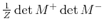
integration (more details can be found in Refs. [17] and [18]. The partition function can be exactly written as,
 |
(312) |
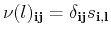
where
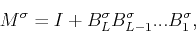 |
(313) |
and
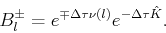 |
(314) |
 is the unit matrix, and
 . Usually the physical observable
  ,
can be expressed in terms of Green's functions for the electrons moving in
the spin field. Then, expressions similar to Eq.(315) can be derived for
the numerator in Eq.(310). Once the partition function is written only
in terms of the spin fields, we can use standard Monte Carlo techniques
(such as Metropolis or heat bath methods) to perform a simulation of the
complicated sums over
that remain to be done. The
probability distribution of a given spin configuration is given in principle
by
,
can be expressed in terms of Green's functions for the electrons moving in
the spin field. Then, expressions similar to Eq.(315) can be derived for
the numerator in Eq.(310). Once the partition function is written only
in terms of the spin fields, we can use standard Monte Carlo techniques
(such as Metropolis or heat bath methods) to perform a simulation of the
complicated sums over
that remain to be done. The
probability distribution of a given spin configuration is given in principle
by
 (unless it becomes negative, see
next section).
(unless it becomes negative, see
next section).
Next: Projector Monte Carlo
Up: Quantum Monte Carlo
Previous: Measurement and averaging
Adrian E. Feiguin
2009-11-04