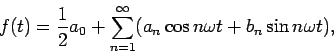
In the previous section we found that the displacement of a particle an be
described as a linear combination of normal modes, i.e. a
superposition of sinusoidal terms. This decomposition of the motion into
various frequencies is more general. It can be shown that any arbitrary
periodic function ![]() of period
of period ![]() can be written as a Fourier series of
sines and cosines:
can be written as a Fourier series of
sines and cosines:
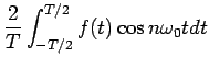 |
(52) | ||
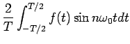 |
(53) |
In general, an infinite number of terms is needed to represent an arbitrary
function ![]() . In practice, a good approximation can usually be obtained
by including a relatively small number of terms.
. In practice, a good approximation can usually be obtained
by including a relatively small number of terms.